Minerals, mining and water
AI and remote sensing from exploration to environmental monitoring · IC-TWEP 2026 workshop
QuestFeed · presented by Dr Firas Alazem
Minerals give every rock a spectral "fingerprint"; satellites read those fingerprints from orbit; and AI models now learn from whole years of satellite data. The same tools that guide exploration also watch what mining does to land and rivers. In this notebook you will work with real data from four generations of satellite sensors and one AI foundation model.
| Step | What you will do | Data |
|---|---|---|
| 1 | Read mineral fingerprints and see what each satellite can resolve | USGS Spectral Library 7 |
| 2 | Map one mining district with four sensors and test whether they agree | Sentinel-2 · ASTER · EMIT · EnMAP |
| 3 | Ask an AI model to find look-alike ground, then teach it to map mining | AlphaEarth Foundations · global mining polygons |
| 4 | Watch mines grow from 1990 to today | Landsat · Sentinel-2 |
| 5 | Trace mining's footprint on rivers | Sentinel-2 |
How to use it: run the cells from top to bottom (Shift + Enter, or Runtime ▸ Run all). You need only a Google account for Colab. Every number comes from real, public data; nothing is simulated.
Step 1 — Every mineral has a spectral fingerprint
Sunlight reflected by a rock carries the imprint of its minerals: chemical bonds absorb light at specific wavelengths. A few absorptions do most of the work in mineral exploration:
| Wavelength | What absorbs | Minerals |
|---|---|---|
| ~0.87–0.93 µm | ferric iron (Fe³⁺) | hematite, goethite, jarosite — weathered sulphides ("gossans") |
| ~2.16–2.21 µm | aluminium–hydroxyl (Al-OH) | kaolinite, alunite, white mica (sericite) — hydrothermal alteration |
| ~2.31–2.35 µm | magnesium–hydroxyl (Mg-OH) and carbonate (CO₃) | chlorite, epidote, serpentine, talc, calcite, dolomite |
The laboratory spectra below come from the USGS Spectral Library. The same spectra are shown as each satellite would record them: a hyperspectral instrument (hundreds of narrow bands, like EMIT and EnMAP), ASTER (six short-wave infrared bands, 2000–2008) and Sentinel-2 (two short-wave infrared bands). Choose three minerals and look at where the fingerprints survive — and where they disappear. The table underneath counts how many bands each sensor places inside each diagnostic window.
# @title Step 1 · Compare mineral fingerprints
MINERAL_1 = "Kaolinite" # @param ["Kaolinite", "Alunite", "Muscovite (sericite)", "Illite", "Montmorillonite", "Pyrophyllite", "Calcite", "Dolomite", "Chlorite", "Epidote", "Serpentine (antigorite)", "Talc", "Hematite", "Goethite", "Jarosite", "Gypsum", "Green vegetation", "Dry grass"]
MINERAL_2 = "Calcite" # @param ["Kaolinite", "Alunite", "Muscovite (sericite)", "Illite", "Montmorillonite", "Pyrophyllite", "Calcite", "Dolomite", "Chlorite", "Epidote", "Serpentine (antigorite)", "Talc", "Hematite", "Goethite", "Jarosite", "Gypsum", "Green vegetation", "Dry grass"]
MINERAL_3 = "Hematite" # @param ["Kaolinite", "Alunite", "Muscovite (sericite)", "Illite", "Montmorillonite", "Pyrophyllite", "Calcite", "Dolomite", "Chlorite", "Epidote", "Serpentine (antigorite)", "Talc", "Hematite", "Goethite", "Jarosite", "Gypsum", "Green vegetation", "Dry grass"]
spectra = fetch_csv("spectra/usgs_mineral_spectra.csv")
meta = {m["name"]: m for m in fetch_json("spectra/spectra_meta.json")["minerals"]}
chosen = [MINERAL_1, MINERAL_2, MINERAL_3]
S2_KEEP = ["B2", "B3", "B4", "B5", "B6", "B7", "B8", "B8A", "B11", "B12"] # surface bands (B1, B9, B10 are atmospheric)
style = {"aviris": ("Hyperspectral (EMIT / EnMAP class)", COLORS["water"], "lines"),
"aster": ("ASTER (2000–2008)", COLORS["dry"], "lines+markers"),
"sentinel2": ("Sentinel-2", COLORS["accent"], "lines+markers")}
fig = make_subplots(rows=3, cols=1, shared_xaxes=True, vertical_spacing=0.06, subplot_titles=[
f"{m} — {meta[m]['diagnostic']}" for m in chosen])
for row, m in enumerate(chosen, start=1):
for sensor, (label, color, mode) in style.items():
d = spectra[(spectra.mineral == m) & (spectra.sensor == sensor)].sort_values("wavelength_um")
if sensor == "sentinel2":
d = d[d.band.isin(S2_KEEP)]
d = d[(d.wavelength_um >= 0.4) & (d.wavelength_um <= 2.5)]
fig.add_trace(go.Scatter(x=d.wavelength_um, y=d.reflectance, mode=mode, name=label, legendgroup=sensor,
showlegend=(row == 1), line=dict(color=color, width=1.6 if sensor == "aviris" else 2),
marker=dict(size=7)), row=row, col=1)
for x0, x1, txt in [(0.85, 0.95, "Fe³⁺"), (2.15, 2.22, "Al-OH"), (2.30, 2.36, "Mg-OH / CO₃")]:
fig.add_vrect(x0=x0, x1=x1, fillcolor="#FDE68A", opacity=0.35, line_width=0, row=row, col=1)
fig.update_xaxes(title_text="wavelength (µm)", row=3, col=1)
fig.update_yaxes(title_text="reflectance")
fig.update_layout(height=820, title="Laboratory fingerprints as three satellites would see them",
**{k: v for k, v in LAYOUT.items() if k != "hovermode"}, hovermode="closest")
fig.show()
# What each sensor can record: how many bands fall inside each diagnostic absorption window?
windows = {"Fe³⁺ 0.85–0.95 µm": (0.85, 0.95), "Al-OH 2.15–2.22 µm": (2.15, 2.22), "Mg-OH / CO₃ 2.30–2.36 µm": (2.30, 2.36)}
rows = []
for sensor in ["aviris", "aster", "sentinel2"]:
d = spectra[(spectra.mineral == MINERAL_1) & (spectra.sensor == sensor)]
if sensor == "sentinel2":
d = d[d.band.isin(S2_KEEP)]
w = d.wavelength_um.values
rows.append({"Sensor": style[sensor][0], **{k: int(((w >= a) & (w <= b)).sum()) for k, (a, b) in windows.items()}})
display(HTML("<b>Bands inside each diagnostic absorption window</b> — a single band can show that light is absorbed, "
"but not the shape of the absorption that identifies a mineral"))
display(pd.DataFrame(rows).set_index("Sensor"))
print("ASTER's two Al-OH bands and one Mg-OH/carbonate band are why its 2000–2008 archive is still used for alteration "
"mapping; Sentinel-2's single, broad 2.19 µm band can flag clays and carbonates together but cannot separate them.")
| Fe³⁺ 0.85–0.95 µm | Al-OH 2.15–2.22 µm | Mg-OH / CO₃ 2.30–2.36 µm | |
|---|---|---|---|
| Sensor | |||
| Hyperspectral (EMIT / EnMAP class) | 11 | 7 | 6 |
| ASTER (2000–2008) | 0 | 2 | 1 |
| Sentinel-2 | 1 | 1 | 0 |
ASTER's two Al-OH bands and one Mg-OH/carbonate band are why its 2000–2008 archive is still used for alteration mapping; Sentinel-2's single, broad 2.19 µm band can flag clays and carbonates together but cannot separate them.
Step 2 — One district, four sensors
Choose a mining district. Each panel shows the same ground mapped by a different generation of sensor:
- Sentinel-2 (10–20 m, 2015 → today): true colour and an iron-oxide index (red ÷ blue) — iron-stained, weathered ground stands out;
- ASTER (15–90 m, short-wave infrared 2000–2008): the Al-OH index (B5 + B7) ÷ B6 — clays and white mica from hydrothermal alteration;
- EMIT (60 m, imaging spectrometer on the International Space Station, 2022 →): NASA's mineral identification, grouped into mineral families;
- EnMAP (30 m, German imaging spectrometer, 2022 →): the depth of the 2.2 µm Al-OH absorption.
Then we ask a scientist's question: do independent sensors agree? The score is an AUC — the chance that a randomly chosen clay or white-mica pixel (according to EMIT) shows a stronger Al-OH signal than a randomly chosen other pixel: 0.5 means no agreement, 1.0 perfect agreement.
# @title Step 2 · Map a district with four sensors
DISTRICT = "Mahd adh Dhahab — Saudi Arabia" # @param ["Mahd adh Dhahab — Saudi Arabia", "Bou Azzer — Morocco", "Sohar–Lasail — Oman", "In Ouzzal (Hoggar) — Algeria"]
districts = {d["label"]: d for d in fetch_json("districts.json")}
D = districts[DISTRICT]
p = f"districts/{D['id']}"
legend = fetch_json(f"{p}/emit_legend.json")
SWIR_COLORS = {"0": "#00000000", "1": "#4FC3F7", "2": "#2E7D32", "3": "#9CCC65", "4": "#F5F5F5", "5": "#CE93D8",
"6": "#FFF176", "7": "#FF8A65", "8": "#90A4AE", "9": "#6D4C41"}
def stretch(a, lo=2, hi=98):
v = a[np.isfinite(a)]
a0, a1 = np.percentile(v, [lo, hi])
return np.clip((a - a0) / (a1 - a0), 0, 1)
def load(rel, band=None):
try:
arr, tr, crs = fetch_raster(f"{p}/{rel}")
return (arr if band is None else arr[band]), tr, crs
except Exception:
return None, None, None
s2_rgb, s2_tr, s2_crs = load("s2_rgb.tif")
s2_idx, _, _ = load("s2_indices.tif")
aster_idx, a_tr, a_crs = load("aster_indices.tif")
emit, e_tr, e_crs = load("emit_minerals.tif")
enmap_bd, n_tr, n_crs = load("enmap_banddepth.tif")
src = fetch_json(f"{p}/sources.json")
fig, ax = plt.subplots(2, 3, figsize=(17, 10))
panels = [
(ax[0, 0], None if s2_rgb is None else np.moveaxis(s2_rgb, 0, -1), None, f"Sentinel-2 true colour · {src.get('s2', {}).get('date', '')}"),
(ax[0, 1], None if s2_idx is None else stretch(s2_idx[0]), "inferno", "Sentinel-2 iron-oxide index (red ÷ blue)"),
(ax[0, 2], None if aster_idx is None else stretch(aster_idx[0]), "viridis", f"ASTER Al-OH index · {src.get('aster', {}).get('date', '')}"),
(ax[1, 1], None if enmap_bd is None else stretch(enmap_bd[0], 5, 99), "magma",
f"EnMAP 2.2 µm Al-OH depth · {src.get('enmap', {}).get('date', '')}\n(20 km window around the mine, outlined in panel 1)"),
]
for a, img, cmap, title in panels:
if img is None:
a.text(0.5, 0.5, "not available for this district", ha="center", va="center", color="#6B7280")
else:
a.imshow(img, cmap=cmap, interpolation="nearest")
a.set_title(title)
a.axis("off")
if enmap_bd is not None and s2_rgb is not None: # outline the EnMAP window on the true-colour panel
from matplotlib.patches import Rectangle
eb = rasterio.transform.array_bounds(*enmap_bd.shape[1:], n_tr)
l, b_, r, t = transform_bounds(n_crs, s2_crs, *eb)
c0, r0 = ~s2_tr * (l, t); c1, r1 = ~s2_tr * (r, b_)
ax[0, 0].add_patch(Rectangle((c0, r0), c1 - c0, r1 - r0, fill=False, edgecolor="white", lw=1.8, ls="--"))
cls = emit[0]
codes = sorted(int(c) for c in legend["swir"])
cmap_e = ListedColormap([SWIR_COLORS[str(c)] for c in codes])
ax[1, 0].set_facecolor("black")
ax[1, 0].imshow(np.ma.masked_equal(cls, 0), cmap=cmap_e, vmin=min(codes) - 0.5, vmax=max(codes) + 0.5, interpolation="nearest")
ax[1, 0].set_title("EMIT mineral families (short-wave infrared)")
ax[1, 0].axis("off")
present = [c for c in codes if c > 0 and (cls == c).mean() > 0.005]
handles = [plt.Rectangle((0, 0), 1, 1, color=SWIR_COLORS[str(c)]) for c in present]
ax[1, 2].legend(handles, [f"{legend['swir'][str(c)]} — {100 * (cls == c).sum() / (cls > 0).sum():.0f} %" for c in present],
loc="center", frameon=False, title="EMIT mineral families in this district", fontsize=10)
ax[1, 2].axis("off")
plt.suptitle(f"{D['name']} — {D['country']}", fontsize=15, fontweight="bold")
plt.tight_layout()
plt.show()
# Do the sensors agree? Bring ASTER and EnMAP onto the EMIT grid and compare their Al-OH signal
# inside EMIT's white-mica / clay classes versus the rest of the district.
def to_emit_grid(arr, tr, crs):
out = np.full(cls.shape, np.nan, np.float32)
reproject(arr.astype(np.float32), out, src_transform=tr, src_crs=crs, src_nodata=np.nan,
dst_transform=e_tr, dst_crs=e_crs, dst_nodata=np.nan, resampling=Resampling.average)
return out
mica_clay = np.isin(cls, [4, 5, 6])
other = (cls > 0) & ~mica_clay
rows = []
reference_ok = (cls == 9).sum() <= 0.5 * (cls > 0).sum() # EMIT must have identified most pixels to serve as the reference
if not reference_ok:
print("EMIT could not identify most pixels in this district ('other' family), so it cannot serve as the reference "
"for the agreement test here — choose another district to see it.")
for name, arr, tr, crs in [("ASTER Al-OH index", None if aster_idx is None else aster_idx[0], a_tr, a_crs),
("EnMAP 2.2 µm depth", None if enmap_bd is None else enmap_bd[0], n_tr, n_crs),
("Sentinel-2 clay proxy (B11 ÷ B12)", None if s2_idx is None else s2_idx[1], s2_tr, s2_crs)]:
if arr is None or mica_clay.sum() < 50 or not reference_ok:
continue
g = to_emit_grid(arr, tr, crs)
ok_in, ok_out = mica_clay & np.isfinite(g), other & np.isfinite(g)
if ok_in.sum() < 30 or ok_out.sum() < 30:
continue
y_true = np.concatenate([np.ones(ok_in.sum()), np.zeros(ok_out.sum())])
auc = roc_auc_score(y_true, np.concatenate([g[ok_in], g[ok_out]]))
rows.append({"Measure": name, "AUC (0.5 = no agreement, 1 = perfect)": round(auc, 2),
"EMIT clay / white-mica pixels": int(ok_in.sum()), "other pixels": int(ok_out.sum())})
if rows:
display(HTML("<b>Do independent sensors agree? How often an EMIT clay / white-mica pixel has a stronger Al-OH signal "
"than a randomly chosen other pixel</b>"))
display(pd.DataFrame(rows).set_index("Measure"))

| AUC (0.5 = no agreement, 1 = perfect) | EMIT clay / white-mica pixels | other pixels | |
|---|---|---|---|
| Measure | |||
| ASTER Al-OH index | 0.77 | 166550 | 452611 |
| EnMAP 2.2 µm depth | 0.87 | 29148 | 61426 |
| Sentinel-2 clay proxy (B11 ÷ B12) | 0.66 | 174908 | 506182 |
Reading the table. ASTER and EnMAP have several narrow bands around 2.2 µm and usually agree with EMIT. Sentinel-2 has only two broad short-wave infrared bands: its clay proxy also responds to moisture, vegetation and other minerals, so it often scores close to 0.5 — a limit of the sensor, not of the method.
Step 3 — An AI that has seen the whole planet
AlphaEarth Foundations (Google DeepMind) condenses a year of optical, radar, thermal, elevation and climate observations into 64 numbers for every 10 m pixel; similar places get similar numbers. We use the openly published 2018 and 2025 layers over Ghana's south-western gold belt — large open-pit mines and widespread artisanal mining (galamsey) along the Ankobra, Offin and Pra rivers.
3a · Similarity search (no training at all). Pick a reference place: its mapped mining ground becomes the reference signature. The map marks the 1 % of the region whose 64-number signatures point most nearly the same way, and we check them against the published mining map.
3b · Teach the AI to map mining. The global mining polygons dataset (Maus et al., 2022) outlines mining areas visible on 2019 imagery. We train a simple classifier on 2025 signatures in the western half of the area and test it on the eastern half it has never seen — honest validation, because neighbouring pixels are near-copies of each other and a random split would flatter the model. Then we apply the same model to 2018 and 2025 to measure how much mining land changed.
# @title Step 3a · Find look-alike ground
REFERENCE = "Artisanal mining on the Offin River near Dunkwa" # @param ["Artisanal mining on the Offin River near Dunkwa", "Artisanal mining on the Ankobra River near Prestea", "Tarkwa open-pit gold mine"]
refs = {r["label"]: r for r in fetch_json("ai/reference_sites.json")}
R = refs[REFERENCE]
emb_q, e_tr, e_crs = fetch_raster("ai/ghana_goldbelt_2025_80m.tif")
valid = emb_q[0] != -128
emb = ((emb_q.astype(np.float32) / 127.5) ** 2) * np.sign(emb_q) # de-quantise → unit vectors
mapped = fetch_raster("ai/ghana_goldbelt_mining_2019_80m.tif")[0][0] == 1 # published mining map (Maus et al. 2022)
from pyproj import Transformer
x, y = Transformer.from_crs("EPSG:4326", e_crs, always_xy=True).transform(R["lon"], R["lat"])
col, row = ~e_tr * (x, y)
r0, c0 = int(row), int(col)
yy, xx = np.mgrid[0:valid.shape[0], 0:valid.shape[1]]
near = ((yy - r0) ** 2 + (xx - c0) ** 2 <= 12 ** 2) & valid # within ~1 km of the place
ref_px = near & mapped if (near & mapped).sum() >= 9 else near # its mapped mining ground
ref = emb[:, ref_px].mean(1)
ref /= np.linalg.norm(ref)
sim = np.tensordot(ref, emb, axes=1)
sim[~valid] = np.nan
top = (sim >= np.nanpercentile(sim[valid], 99)) & valid # the 1 % most similar ground
rgb_q, r_tr, _ = fetch_raster("ai/ghana_goldbelt_s2_rgb.tif")
img = np.moveaxis(rgb_q, 0, -1)
fig, ax = plt.subplots(1, 2, figsize=(15, 8))
ax[0].imshow(img)
ax[0].set_title("Sentinel-2 true colour, dry season 2025–26")
ax[1].imshow(img.mean(2), cmap="gray", vmin=0, vmax=255)
ax[1].imshow(np.ma.masked_where(~top, top), cmap=ListedColormap(["#FACC15"]), interpolation="nearest")
ax[1].contour(mapped.astype(float), levels=[0.5], colors="#22D3EE", linewidths=0.5)
ax[1].plot(c0, r0, marker="*", color="#E4572E", markersize=18, markeredgecolor="k")
ax[1].set_title(f"Yellow: 1 % most similar to {REFERENCE}\n(cyan = mapped mining areas, star = reference)")
for a in ax:
a.axis("off")
plt.tight_layout()
plt.show()
px_km2 = (abs(e_tr.a) / 1000) ** 2
share, base = 100 * mapped[top].mean(), 100 * mapped[valid].mean()
print(f"The 1 % most similar ground ({top.sum() * px_km2:,.0f} km² of {valid.sum() * px_km2:,.0f} km²): {share:.0f} % of it is "
f"mapped mining — {share / base:.1f} × the share across the whole region ({base:.0f} %).")

The 1 % most similar ground (95 km² of 9,468 km²): 87 % of it is mapped mining — 7.1 × the share across the whole region (12 %).
# @title Step 3b · Teach the AI to map mining, test it honestly, measure change 2018 → 2025
labels, l_tr, _ = fetch_raster("ai/ghana_goldbelt_mining_2019_80m.tif") # 1 = mapped mining area (2019)
mine = labels[0] == 1
emb18_q = fetch_raster("ai/ghana_goldbelt_2018_80m.tif")[0]
emb18 = ((emb18_q.astype(np.float32) / 127.5) ** 2) * np.sign(emb18_q)
ok = valid & (emb18_q[0] != -128)
rng = np.random.default_rng(42)
H, W = mine.shape
west = np.zeros_like(mine); west[:, : W // 2] = True
def sample(region, n_pos=3000, n_neg=9000):
pos = np.flatnonzero(region & ok & mine); neg = np.flatnonzero(region & ok & ~mine)
pos = rng.choice(pos, min(n_pos, pos.size), replace=False); neg = rng.choice(neg, min(n_neg, neg.size), replace=False)
idx = np.concatenate([pos, neg])
return emb.reshape(64, -1)[:, idx].T, np.concatenate([np.ones(pos.size), np.zeros(neg.size)])
Xtr, ytr = sample(west)
Xte, yte = sample(~west)
clf = LogisticRegression(max_iter=2000, C=1.0).fit(Xtr, ytr)
pte = clf.predict_proba(Xte)[:, 1]
print(f"Trained on {len(ytr):,} pixels in the west; tested on {len(yte):,} unseen pixels in the east.")
print(f"East-half test: AUC {roc_auc_score(yte, pte):.3f} · precision {precision_score(yte, pte > 0.5):.2f} · "
f"recall {recall_score(yte, pte > 0.5):.2f}")
prob25 = clf.predict_proba(emb.reshape(64, -1).T)[:, 1].reshape(H, W)
prob18 = clf.predict_proba(emb18.reshape(64, -1).T)[:, 1].reshape(H, W)
m25, m18 = (prob25 > 0.5) & ok, (prob18 > 0.5) & ok
new = m25 & ~m18
fig, ax = plt.subplots(1, 3, figsize=(18, 7))
ax[0].imshow(np.where(ok, prob25, np.nan), cmap="YlOrRd", vmin=0, vmax=1, interpolation="nearest")
ax[0].contour(mine.astype(float), levels=[0.5], colors="cyan", linewidths=0.4)
ax[0].set_title("AI mining probability, 2025 (cyan = mapped 2019)")
ax[1].imshow(np.where(m18, 1, np.nan), cmap=ListedColormap(["#6D4C41"]), interpolation="nearest")
ax[1].set_title("AI-mapped mining land, 2018")
ax[2].imshow(np.where(m18 & m25, 1, np.nan), cmap=ListedColormap(["#BDBDBD"]), interpolation="nearest")
ax[2].imshow(np.where(new, 1, np.nan), cmap=ListedColormap(["#E53935"]), interpolation="nearest")
ax[2].set_title("2025: unchanged mining (grey), new since 2018 (red)")
for a in ax:
a.axis("off")
plt.tight_layout()
plt.show()
print(f"AI-mapped mining land: {m18.sum() * px_km2:,.0f} km² in 2018 → {m25.sum() * px_km2:,.0f} km² in 2025 "
f"({100 * (m25.sum() - m18.sum()) / max(m18.sum(), 1):+.0f} %); newly mined since 2018: {new.sum() * px_km2:,.0f} km².")
print("Read these as model estimates with the test scores above as their quality label — not as an official inventory.")
Trained on 12,000 pixels in the west; tested on 12,000 unseen pixels in the east. East-half test: AUC 0.932 · precision 0.80 · recall 0.65

AI-mapped mining land: 547 km² in 2018 → 1,219 km² in 2025 (+123 %); newly mined since 2018: 715 km². Read these as model estimates with the test scores above as their quality label — not as an official inventory.
Step 4 — Watching mines grow, 1990 → today
The Landsat archive reaches back to the 1980s and Sentinel-2 adds 10 m detail from 2015. Together they let anyone watch a mine open, expand and — sometimes — close. Choose a site to play its time-lapse.
# @title Step 4 · Mine time-lapses
SITE = "Gara Djebilet iron ore — Algeria" # @param ["Gara Djebilet iron ore — Algeria", "Djebel Onk phosphate — Algeria", "Khouribga phosphate basin — Morocco", "Abu Tartur phosphate — Egypt", "Mansourah-Massarah gold — Saudi Arabia", "Lasail copper (Sohar) — Oman", "Hajar mountain quarries, Ras Al Khaimah — United Arab Emirates", "Tarkwa gold — Ghana", "Simandou iron ore — Guinea"]
from IPython.display import Image as _Image
mines = {m["label"]: m for m in fetch_json("mines.json")}
M = mines[SITE]
display(HTML(f"<b>{M['name']}</b> — {M['country']}. {M.get('note', '')}"))
display(_Image(url=f"{STORE}/mines/{M['id']}/timelapse.gif", width=760))
frames = fetch_csv(f"mines/{M['id']}/frames.csv")
display(frames[["year", "sensor", "date"]].set_index("year").T)
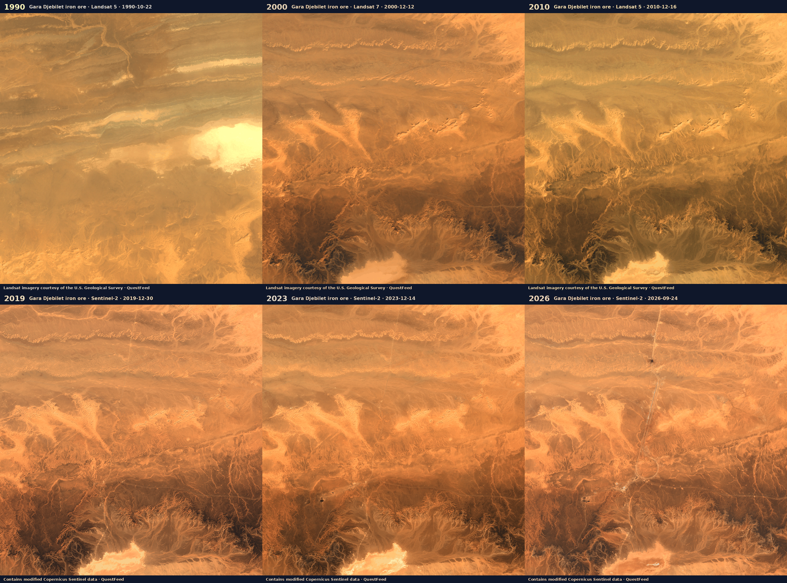
| year | 1990 | 1995 | 2000 | 2005 | 2010 | 2014 | 2017 | 2019 | 2021 | 2023 | 2025 | 2026 |
|---|---|---|---|---|---|---|---|---|---|---|---|---|
| sensor | landsat-5 | landsat-5 | landsat-7 | landsat-5 | landsat-5 | landsat-8 | sentinel-2a | sentinel-2b | sentinel-2b | sentinel-2a | sentinel-2b | sentinel-2b |
| date | 1990-10-22 | 1995-06-14 | 2000-12-12 | 2005-07-11 | 2010-12-16 | 2014-11-25 | 2017-06-18 | 2019-12-30 | 2021-12-29 | 2023-12-14 | 2025-11-28 | 2026-09-24 |
Step 5 — Mining and rivers
Artisanal mining moves sediment straight into rivers. Clear water looks dark in Sentinel-2's red band; water carrying suspended clay and silt reflects much more red light. Measuring the red reflectance of the river surface in the dry season each year gives a consistent, independent record of river condition — along rivers that also cross borders: the Tano flows on into Côte d'Ivoire.
# @title Step 5 · River condition from space
rivers = fetch_csv("rivers/river_red_reflectance.csv")
fig = go.Figure()
for reach, d in rivers.groupby("reach"):
fig.add_trace(go.Scatter(x=d["season"], y=d["red_reflectance_median"], mode="lines+markers", name=reach))
fig.update_layout(title="Dry-season red reflectance of the river surface (higher = more suspended sediment)",
yaxis_title="red reflectance", height=430, **LAYOUT)
fig.show()
first, last = rivers["season"].min(), rivers["season"].max()
print("Seasons without enough cloud-free images are left blank — dry-season cumulus is common over the forest.")
for reach, d in rivers.groupby("reach"):
d = d.dropna(subset=["red_reflectance_median"])
a, b = d.iloc[0], d.iloc[-1]
print(f"{reach}: {a['red_reflectance_median']:.3f} ({a['season']}) → {b['red_reflectance_median']:.3f} ({b['season']})")
before, _, _ = fetch_raster("rivers/before.tif")
after, _, _ = fetch_raster("rivers/after.tif")
info = fetch_json("rivers/before_after.json")
fig, ax = plt.subplots(1, 2, figsize=(15, 6.5))
ax[0].imshow(np.moveaxis(before, 0, -1)); ax[0].set_title(f"{info['reach']} · {info['before_date']}")
ax[1].imshow(np.moveaxis(after, 0, -1)); ax[1].set_title(f"{info['reach']} · {info['after_date']}")
for a in ax:
a.axis("off")
plt.tight_layout()
plt.show()
Seasons without enough cloud-free images are left blank — dry-season cumulus is common over the forest. Ankobra River near Prestea: 0.145 (2018-19) → 0.222 (2024-25) Offin River at Dunkwa-on-Offin: 0.200 (2016-17) → 0.202 (2025-26) Pra River near Twifo Praso: 0.233 (2016-17) → 0.243 (2025-26) Tano River near Elubo (Côte d'Ivoire border): 0.165 (2017-18) → 0.175 (2024-25)

What you just did
- Read mineral fingerprints and saw why the number and placement of bands matters;
- mapped a mining district with four sensors and checked that independent instruments agree;
- used a foundation AI model for similarity search, trained a mining classifier and validated it on ground it had never seen, then measured change between 2018 and 2025;
- watched mines grow over three decades;
- followed mining's footprint into rivers.
Limits to keep in mind. Satellite mineral maps show the surface, not what lies below; identifications from space need field and laboratory confirmation; AI estimates carry the quality measured on the hold-out, no more. Used well, these tools tell you where to look first — for new resources and for environmental risk — at a fraction of the cost of covering the ground on foot.
Take it further with the take-home notebooks: a transparent prospectivity map checked honestly against known mining areas, a hyperspectral deep dive with real EnMAP spectra, and structural mapping from elevation data.
Data sources
- USGS Spectral Library Version 7 — Kokaly, R.F. et al. (2017) USGS Data Series 1035 (public domain).
- Sentinel-2 L2A — contains modified Copernicus Sentinel data (ESA), via Earth Search on AWS.
- ASTER L1T — NASA/METI, via Microsoft Planetary Computer.
- EMIT L2B mineral identification — NASA JPL / LP DAAC. NASA notes that identifications beyond its ten core minerals require further validation, particularly for resource exploration.
- EnMAP L2A — © DLR, contains modified EnMAP data.
- AlphaEarth Foundations Satellite Embedding — produced by Google and Google DeepMind (CC-BY 4.0).
- Global-scale mining polygons v2 — Maus, V. et al. (2022) PANGAEA (CC BY-SA 4.0).
- Landsat — courtesy of the U.S. Geological Survey.
Prepared by QuestFeed for IC-TWEP 2026, University of Tlemcen. questfeed.com